
1. Introduction
When we want to record an audio or an image to our phones, the analog sensors capture the audio and an image as a continuous-time signal. We convert these signals into digital signals that we can store and access later. When we want to play the audio in a speaker or show the image on a monitor, we reconstruct the original continuous-time signal from the stored digital signal. We can use the sampling theorem to reconstruct the original signal from the discrete one. There are two steps to reconstruct the signal: apply a sequence of impulses to the samples x(n),
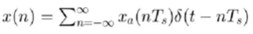
and use a reconstruction filter,

When we sampled signal, we need to choose the correct sampling frequency to prevent aliasing. Aliasing happen when the discrete-time signal produce ”aliases” of the continuous signal. The sampling frequency should be consistent with the Nyquist rate. The Nyquist rate established the minimum sampling frequency, which is fs > 2fm. In this blog, we discuss aliasing by examining the reconstructed signal at different sampling frequency.
2. Aliasing
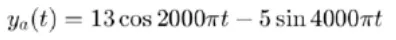
Consider the continuous-time signal,

The frequencies existing in the signal are f1 = 2 kHz, f2 = 6 kHz, and f1 = 12 kHz. Hence the signal has multiple frequency component; we choose the maximum frequency as our basis for the sampling frequency. As we stated earlier, the sampling frequency should follow fs > 2fm. The Nyquist rate is 24 kHz. The ideal sampling frequency to prevent aliasing is greater than or equal to 24 kHz.
We can have the discrete-time signal,
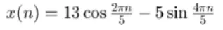
for the continuous-time signal at 5 kHz sampling frequency. If we have only 1 kHz and 2 kHz component in our reconstructed signal. We have the reconstructed signal,
which is different from the original signal. It is due to low sampling frequency that causes aliasing in the reconstruction. When the sampling frequency is below the the Nyquist rate aliasing occurs. The signal missed out a lot of the frequency component from the original signal. It is shown in the reconstructed signal where it is not the same with the continuous-time signal.
Aliasing is often not desired, but it has a practical application we can't deny. Signal sampling in our oscilloscope exploits the aliasing effects to map high frequency signal in lower frequency. To elaborate, when the frequency component of the signal is larger than the bandwidth B, it results to aliasing of the reconstructed signal. If the sampling is fs > 2B, but fs < B the signal contains the aliases of frequencies ranging 0 < f < fs/2. These signals are often called band pass or narrow band pass.
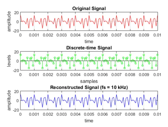
When we increase the sampling frequency to 10 kHz, we see that the reconstructed signal is closed to the original signal, but we can see some aliases on it. When the sampling frequency is below the Nyquist rate, we can expect aliasing to occur.
close all; clear all; clc;

fs = 10000;
Ts = 1/fs;
n0 = 2000*pi*Ts;
n1 = 6000*pi*Ts;
n2 = 12000*pi*Ts;

t = 0:Ts:0.01;
xat = 3*cos(2000*pi*t)+5*sin(6000*pi*t)+10*cos(12000*pi*t);

n = 0:1:fs*0.01;
xn = 3*cos(n0*n)+5*sin(n1*n)+10*cos(n2*n);

for i = 1:length(t)
    h(i) = sinc(pi*t(i)/Ts);
end

xt = 0;
Xt = [];
sum_Xt = 0;
for j = 1:length(n)
    xt = xn*h(j);
    sum_Xt = sum_Xt+xt;
    Xt = [Xt; {xt}];
end
figure;
ax1 = subplot(3,1,1);
plot(t,xat, 'r');hold on; grid on;
ax2 = subplot(3,1,2);
stem(t,xn, 'g','MarkerSize', 4); hold on; grid on;
ax3 = subplot(3,1,3);
plot(t,sum_Xt, 'b');hold on; grid on;
xlabel(ax1, 'time');ylabel(ax1, 'amplitude');
title(ax1, 'Original Signal')
xlabel(ax2, 'samples');ylabel(ax2, 'levels');
title(ax2, 'Discrete-time Signal');
xlabel(ax3, 'time');ylabel(ax3, 'amplitude');
title(ax3, 'Reconstructed Signal (fs = 10 kHz)');
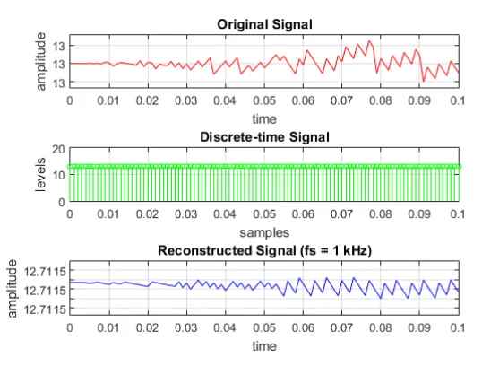
To elaborate on aliasing occurrence at the sampling frequency below the Nyquist rate, we set the sampling frequency to 1 kHz and 2 kHz. At 1 kHz, we can see that the reconstructed signal do not have same frequency component as to the original one. The reconstructed signal contains only the lower frequency components of the original signal.
close all; clear all; clc;

fs = 1000;
Ts = 1/fs;
n0 = 2000*pi*Ts;
n1 = 6000*pi*Ts;
n2 = 12000*pi*Ts;

t = 0:Ts:0.1;
xat = 3*cos(2000*pi*t)+5*sin(6000*pi*t)+10*cos(12000*pi*t);

n = 0:1:fs*0.1;
xn = 3*cos(n0*n)+5*sin(n1*n)+10*cos(n2*n);

for i = 1:length(t)
    h(i) = sinc(pi*t(i)/Ts);
end

xt = 0;
Xt = [];
sum_Xt = 0;
for j = 1:length(n)
    xt = xn*h(j);
    sum_Xt = sum_Xt+xt;
    Xt = [Xt; {xt}];
end
figure;
ax1 = subplot(3,1,1);
plot(t,xat, 'r');hold on; grid on;
ax2 = subplot(3,1,2);
stem(t,xn, 'g','MarkerSize', 4); hold on; grid on;
ax3 = subplot(3,1,3);
plot(t,sum_Xt, 'b');hold on; grid on;
xlabel(ax1, 'time');ylabel(ax1, 'amplitude');
title(ax1, 'Original Signal')
xlabel(ax2, 'samples');ylabel(ax2, 'levels');
title(ax2, 'Discrete-time Signal');
xlabel(ax3, 'time');ylabel(ax3, 'amplitude');
title(ax3, 'Reconstructed Signal (fs = 1 kHz)');
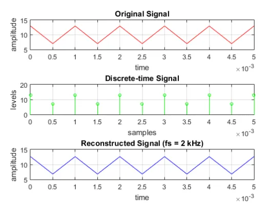
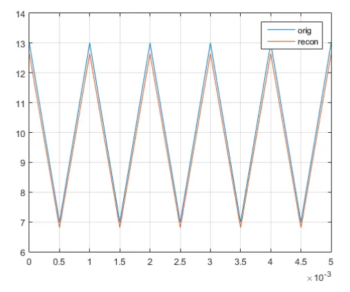
At 2 kHz, the reconstructed signal still an alias of the original signal. We can see in the plot below that it has same frequency component as to the original signal, but the reconstructed signal is shifted below the original signal. There are two important observation we can draw out from aliasing at a sampling frequency lower than Nyquist rate. First, the signal contains only the lower frequency component of the original. It works similar to a band pass filter rather than reconstructing the signal. Second, the signal may have similar orientation to original signal, but contains lower frequency than the original signal.
close all; clear all; clc;

fs = 2000;
Ts = 1/fs;
n0 = 2000*pi*Ts;
n1 = 6000*pi*Ts;
n2 = 12000*pi*Ts;

t = 0:Ts:0.005;
xat = 3*cos(2000*pi*t)+5*sin(6000*pi*t)+10*cos(12000*pi*t);

n = 0:1:fs*0.005;
xn = 3*cos(n0*n)+5*sin(n1*n)+10*cos(n2*n);

for i = 1:length(t)
    h(i) = sinc(pi*t(i)/Ts);
end

xt = 0;
Xt = [];
sum_Xt = 0;
for j = 1:length(n)
    xt = xn*h(j);
    sum_Xt = sum_Xt+xt;
    Xt = [Xt; {xt}];
end
figure;
ax1 = subplot(3,1,1);
plot(t,xat, 'r');hold on; grid on;
ax2 = subplot(3,1,2);
stem(t,xn, 'g','MarkerSize', 4); hold on; grid on;
ax3 = subplot(3,1,3);
plot(t,sum_Xt, 'b');hold on; grid on;
xlabel(ax1, 'time');ylabel(ax1, 'amplitude');
title(ax1, 'Original Signal')
xlabel(ax2, 'samples');ylabel(ax2, 'levels');
title(ax2, 'Discrete-time Signal');
xlabel(ax3, 'time');ylabel(ax3, 'amplitude');
title(ax3, 'Reconstructed Signal (fs = 2 kHz)');

figure;
plot(t,xat); hold on; grid on;
plot(t,sum_Xt); grid on;legend('orig','recon')
We increase the sampling frequency to 15 kHz, and observe the reconstructed signal if aliasing still occurs. When the sampling frequency is above the Nyquist rate, we can expect that the signal is accurately reconstructed. As shown in the plot below, the reconstructed signal is the same as to the original signal. However, we note that the signal may loss some amplitude value due to interpolation.
close all; clear all; clc;

fs = 15000;
Ts = 1/fs;
n0 = 2000*pi*Ts;
n1 = 6000*pi*Ts;
n2 = 12000*pi*Ts;

t = 0:Ts:0.005;
xat = 3*cos(2000*pi*t)+5*sin(6000*pi*t)+10*cos(12000*pi*t);

n = 0:1:fs*0.005;
xn = 3*cos(n0*n)+5*sin(n1*n)+10*cos(n2*n);

for i = 1:length(t)
    h(i) = sinc(pi*t(i)/Ts);
end

xt = 0;
Xt = [];
sum_Xt = 0;
for j = 1:length(n)
    xt = xn*h(j);
    sum_Xt = sum_Xt+xt;
    Xt = [Xt; {xt}];
end
figure;
ax1 = subplot(3,1,1);
plot(t,xat, 'r');hold on; grid on;
ax2 = subplot(3,1,2);
stem(t,xn, 'g','MarkerSize', 4); hold on; grid on;
ax3 = subplot(3,1,3);
plot(t,sum_Xt, 'b');hold on; grid on;
xlabel(ax1, 'time');ylabel(ax1, 'amplitude');
title(ax1, 'Original Signal')
xlabel(ax2, 'samples');ylabel(ax2, 'levels');
title(ax2, 'Discrete-time Signal');
xlabel(ax3, 'time');ylabel(ax3, 'amplitude');
title(ax3, 'Reconstructed Signal (fs = 15 kHz)');

figure;
plot(t,xat); hold on; grid on;
plot(t,sum_Xt, '--'); grid on;legend('orig','recon');
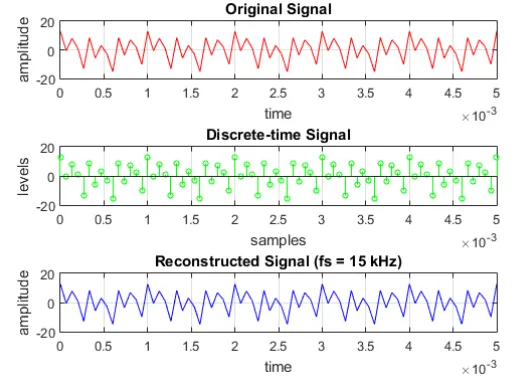
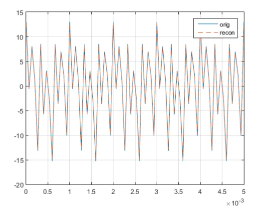
The reconstructed signal has a minimal error as compared to the original signal. It is not due to aliasing, but to the error innate in interpolating the signal. Aliasing occurs when we take few samples from the signal or we sampled the signal too slow. The minimum sampling rate is defined by the Nyquist rate so that we can accurately reconstruct the signal. When the sampling frequency is below the Nyquist rate, the reconstructed signal is an alias to the original continuous-time signal. When aliasing happen, our reconstructed signal only has the lower frequency component of the original signal.
3. Conclusion
When we sampled signal, we should adhere to the Nyquist rate so that we prevent aliasing. Aliasing happen when the discrete-time signal produce ”aliases” of the continuous signal. Nyquist rate establishes the minimum sampling frequency, which is fs > 2fm. If the sampling signal is below the Nyquist rate, we can expect aliasing to happen, and the reconstructed signal contains only the lower frequency component of the original. In contrast, we have a good reconstruction when the sampling frequency adhere to the Nyquist rate.
4. References
Neal S. Widmer, Gregory L. Moss, Ronald J. Tocci, Digital Systems: Principles and Applications, 12th Edition, online access
Gérard Blanchet, Maurice Charbit, Digital Signal and Image Processing Using MATLAB, online access
John W. Leis, Digital Signal Processing Using MATLAB for Students and Researchers. online access