
Excel syntax for INDEX(): |
|---|
=INDEX(array, row_num[, column_num]) |
Excel syntax for MATCH(): |
|---|
=MATCH(lookup_value, lookup_array, [match_type]) |
| Syntax for INDEX-MATCH: |
|---|
=INDEX(array, MATCH(lookup_value, lookup_array, [match_type]) [, MATCH(lookup_value, lookup_array, [match_type])]) |
As convenient as VLOOKUP() is, it has a limitation: it can't look for data to it's left. For that reason, INDEX-MATCH is a more versatile way to rewrite nested IF()s. EUR in D6 will use INDEX-MATCH.
The MATCH() portion of INDEX-MATCH is nearly identical to that used for CHOOSE-MATCH. The only change is setting B6 equal to EUR.
Referring to the tables at the top of this post, these are the values needed by INDEX() in cell D6:
INDEX() item | Cell(s) or range | Value | Comments |
|---|---|---|---|
array | $H$3:$H$10 | Rates | Column 2 of the Exchange Rates table |
row_num | See Comments | See Comments | Result from MATCH() is fed to row_num |
[column_num] | See Comments | See Comments | Result from MATCH() is fed to row_num |
Just as multiplication tables are used to find products of 2 numbers, INDEX() is used to find the value at the intersection of row_num and (the optional) column_num. In this case, it’s even easier since only 1 column of the Exchange Rates table is used,so the revised syntax for INDEX-MATCH looks like this:
| REVISED Syntax for INDEX-MATCH: |
|---|
=INDEX(array, MATCH(lookup_value, lookup_array, [match_type])) |
These are the revised values for INDEX():
INDEX() item | Cell(s) or range | Value | Comments |
|---|---|---|---|
array | $H$3:$H$10 | Rates | Column 2 of the Exchange Rates table |
row_num | See Comments | See Comments | Result from MATCH() is fed to row_num |
[column_num] | N/A | N/A | Optional, and not needed here |
Replace row_num from the INDEX() below with the MATCH() above, and the contents of D6 should look like this:
| REVISED INDEX-MATCH for D6: |
|---|
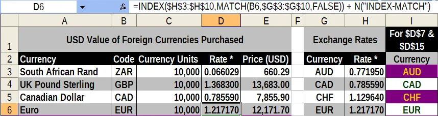
=INDEX($H$3:$H$10, MATCH(B6, $G$3:$G$10, FALSE)) |
Note that B6 is set to EUR, MATCH() determined that it is listed 3rd in Column 1 of the Exchange Rates table, and INDEX() used that detail to determine that its corresponding rate in Column 2 is 1.217170.
This excerpt is taken from 8 Ways To Rewrite Nested IF() Functions at Magna Carta XLS Communications. Each of the 8 nested IF() rewrites from that post will be featured in its own post here.
Other posts will be migrated to this blog before I begin writing posts natively here.