
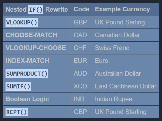
There are numerous ways of rewriting convoluted nested IF()s, only 8 of which are covered here to accommodate versions of Excel going back to 2000.
Some rewrites use just 1 function. VLOOKUP() is the best-known of the single functions used for rewriting nested IF()s. SUMPRODUCT(), however, is the most powerful due to its number-crunching prowess. In the case of Rewrite #8 (REPT()), the function is used repeatedly.
Some rewrites use 2-function formulas. Among these are the more commmonly used INDEX-MATCH and the lesser known VLOOKUP-CHOOSE. While INDEX-MATCH is preferred because it avoids a limitation of VLOOKUP(), VLOOKUP-CHOOSE lets VLOOKUP() “look to the left,” and therefore overcome that limitation.
If you can believe it, one nested IF() rewrite uses zero functions: Boolean Logic (Rewrite #7). Instead, this rewrite uses a series of comparisons, each producing a 1 or a 0, to be multiplied by corresponding values in order to produce the final answer. Rewrite #8 (REPT()) closely follows this format.
Below are the nested IF() rewrites explained earlier (plus the nested IF() which inspired them):
Nested IF()s
| =IF(B3=$G$3, $H$3, IF(B3=$G$4, $H$4, IF(B3=$G$5, $H$5, IF(B3=$G$6, $H$6, IF(B3=$G$7, $H$7, IF(B3=$G$8, $H$8, IF(B3=$G$9, $H$9, IF(B3=$G$10, $H$10)))))))) |
|---|
Situations like this one are why nested IF() rewrites are needed. |
Nested IF()s using ZAR (South African Rand)
Rewrite #1 — VLOOKUP()
| =VLOOKUP(B4, $G$3:$H$10, 2, FALSE) |
|---|
| One function is used. |
Rewrite #1 using GBP (UK Pound Sterling)
Rewrite #2 — CHOOSE-MATCH
| =CHOOSE(MATCH(B5, $G$3:$G$10, FALSE), $H$3, $H$4, $H$5, $H$6, $H$7, $H$8, $H$9, $H$10) |
|---|
| Two-function formula is used. |
Rewrite #2 using CAD (Canadian Dollar)
Rewrite #3 — INDEX-MATCH
| =INDEX($H$3:$H$10, MATCH(B6, $G$3:$G$10, FALSE)) |
|---|
Two-function formula is used. In this case, this is the most common for nested IF() rewrites. |
Rewrite #3 using EUR (Euro)
Rewrite #4 — VLOOKUP-CHOOSE
| =VLOOKUP($B$7, CHOOSE({1,2}, $I$3:$I$10, $H$3:$H$10), 2, FALSE) |
|---|
| Two-function formula is used. Not as common as INDEX-MATCH, this rewrite shows how VLOOKUP can overcome its best-known limitation. |
Rewrite #4 using CHF (Swiss Franc)
Rewrite #5 — SUMPRODUCT()
| =SUMPRODUCT(--(B8=$G$3:$G$10), $H$3:$H$10) |
|---|
One function is used. When used with numeric data, SUMPRODUCT() is the most powerful way to rewrite a nested IF() |
Rewrite #5 using AUD (Australian Dollar)
Rewrite #6 — SUMIF()
| =SUMIF($G$3:$G$10, B9, $H$3:$H$10) |
|---|
One function is used. SUMIF() is considered an enhanced SUM() function. |
Rewrite #6 using XCD (East Caribbean States Dollar)
Rewrite #7 — Boolean Logic
| =(B10=$G$3)$H$3 + (B10=$G$4)$H$4 + (B10=$G$5)$H$5 + (B10=$G$6)$H$6 + (B10=$G$7)$H$7 + (B10=$G$8)$H$8 + (B10=$G$9)$H$9 + (B10=$G$10)$H$10 |
|---|
| Zero functions are used. Instead, a series of comparisons are made and muliplied by numeric values to obtain the final answer. |
Rewrite #7 using INR (Indian Rupee)
Rewrite #8 —REPT()
| =1 * ( REPT($H$3,(B11=$G$3)) & REPT($H$4,(B11=$G$4)) & REPT($H$5,(B11=$G$5)) & REPT($H$6,(B11=$G$6)) & REPT($H$7,(B11=$G$7)) & REPT($H$8,(B11=$G$8)) & REPT($H$9,(B11=$G$9)) & REPT($H$10,(B11=$G$10)) ) |
|---|
One function is used– repeatedly, in a way similar to Boolean Logic. Since REPT() is normally used with text, the final output from this series of REPT() calls needs to be multiplied by 1 for use as a number later. |
Rewrite #8 using GBP (UK Pound Sterling)
Certain nested IF() rewrites are better-suited for certain situations (especially if text is involved). While certain nested IF() rewrites are preferred over others, all nested IF() rewrites are worth knowing.
This excerpt is taken from 8 Ways To Rewrite nested IF() Functions at Magna Carta XLS Communications. Each of the 8 nested IF() rewrites from that post will be featured in its own post here.
Other posts will be migrated to this blog before I begin writing posts natively here.